2. Picture Plane#
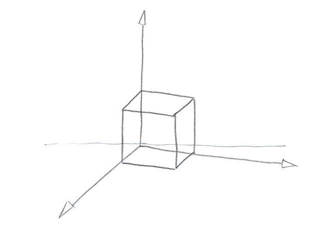
Architectural notation does not define the position of a camera in 3D space, but rather focuses on the aspect of the figure as it appears after the projection. The conventional method to define the picture is by setting three variables: the directions of the coordinate axes. The axes are represented in their projection, and are defined by the angles between Oz/Ox, Oz/Oy and Ox/Oy.
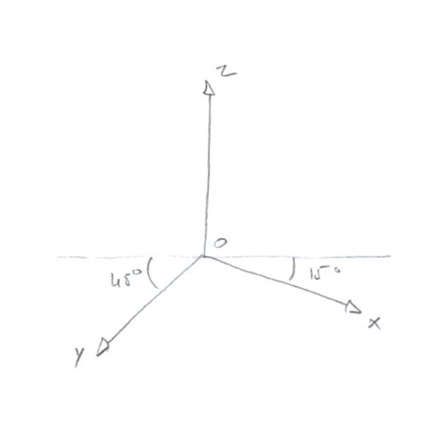
The three angles are corelated (Oz/Ox + Oz/Oy + Ox/Oy == 360°) and the Oz axis is positioned vertically in most cases. The notation is simplified by only using the Oz/Ox and Oz/Oy angles and by substract 90° from their values. The image presents an “15/45” axonometry. The goal of the Pohlke add-on is to implement this notation system. The interface provides the user a way to define a specific projection view by setting these two values, the alpha and beta angles.
2.1. Axonometric Projection#
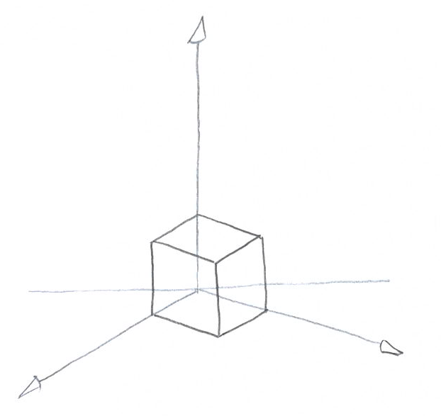
Knowing on which conventions architectural notation is relying, we can see how boht systems are correlated. In both cases, we are in front of a prjection plane, positioned somewhere in 3D space. The architectural system, manipulates this plane via the projected angles of the 3D space reference axes. In other words, in a modeling space with a camera, the projection is executed when shoting an image with the camera. Likewise, the axonometric projection relies on a picture plane positioned in space and the scene is projected perpendicularly onto the plane.[1]
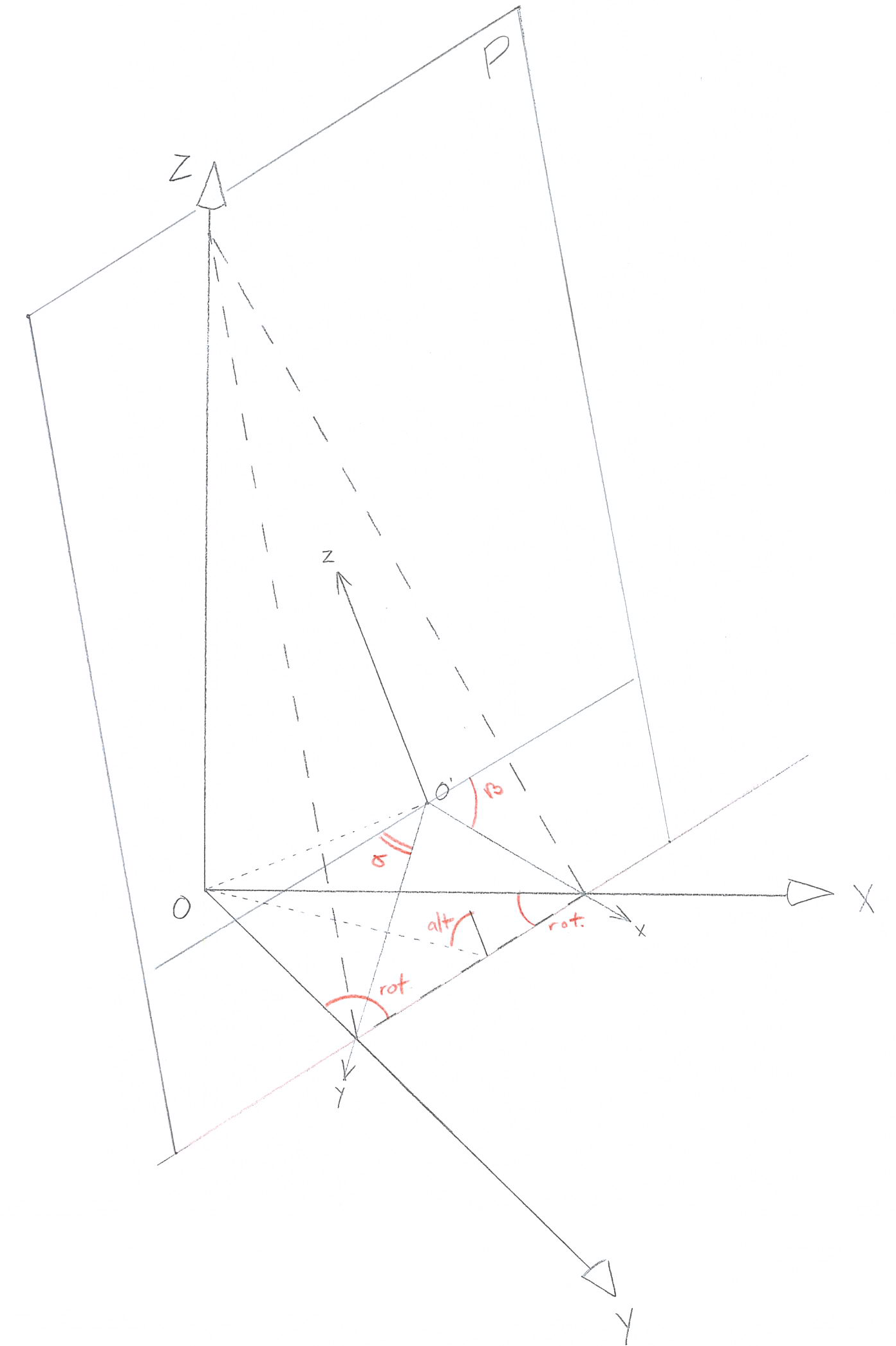
The angles alpha & beta are the result of a certain position in space of the picture plane. Modifying the alpha & beta values is a way of moving the picture plane in space.
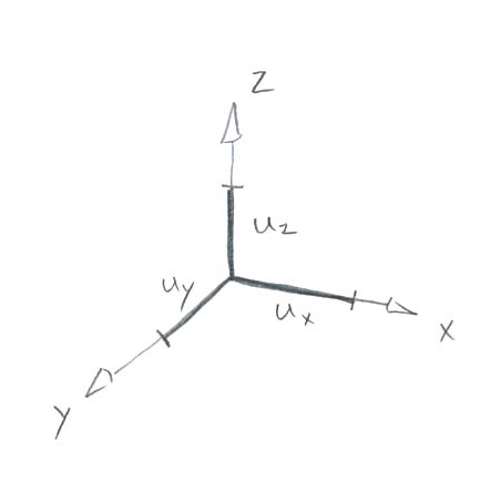
Likewise, changing the alpha & beta angles are a way to modify the properties of the projected image. Namely, projections present certain deformations which are the reduction coefficients of the singles axes.
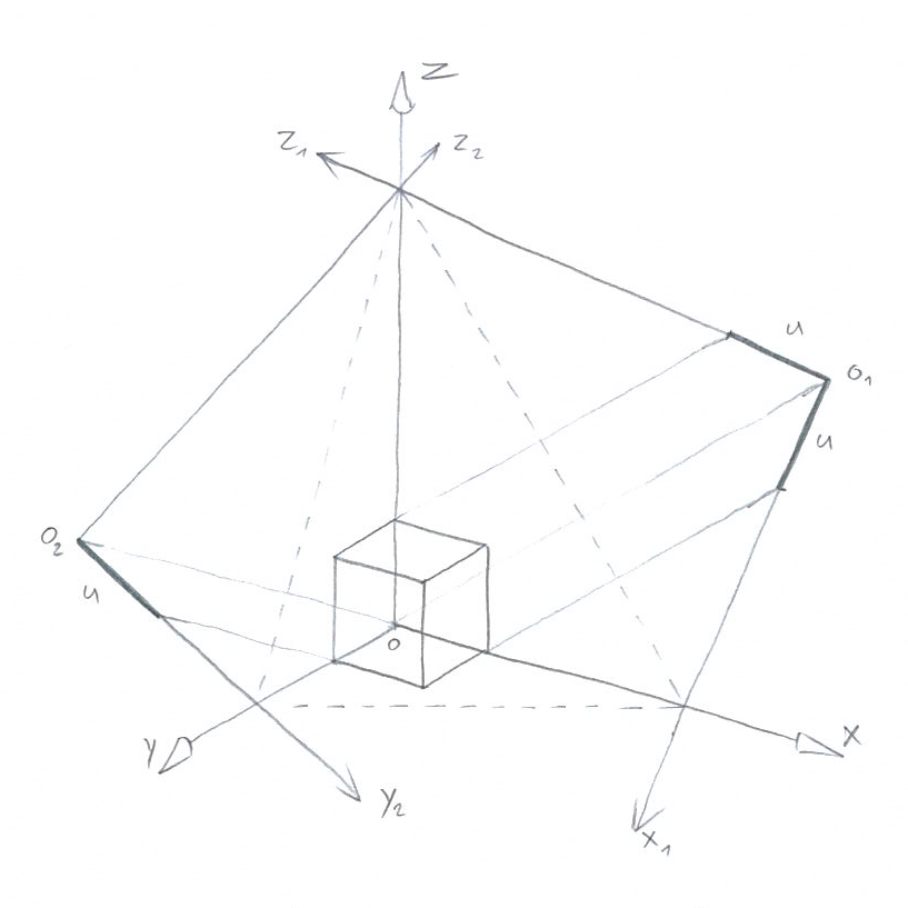
An axonometric projection has different scale factors for each axis. As, shown in the image, a unitary vector of u = 1, when projected in (trimetric) axonometry, has a different shortening for each axis. The projected figure follows a set of geometric properties depending on the position of the picture plane. These properties are one to one linked with the rotation and altitude angles. For each alpha/beta angle pair, only one resulting projection exists. All axonometric projections can be assigned to one of three cases: trimetric, dimetric and isometric.
2.1.1. Isometric#
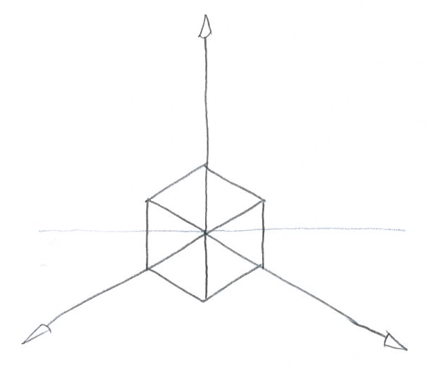
alpha, beta = 30, 30
Projection in which the picture plane forms the same angle with each of the three axes Ox, Oy, Oz.
This position of the picture plane is reflected in the axonometry by the equality of the three angles formed between the axonometric images of the three axes.
120° 120° 120°The three reduction coefficients are identical.
x=1.00 y=1.00 z=1.00
2.1.2. Dimetric#
alpha, beta = 41.5, 7
Projection in which the picture plane forms the same angle with two of the three axes Ox, Oy, Oz.
This position of the picture plane is reflected in the axonometry by the equality of two of the angles formed between the axonometric images of the three axes.
131.5° 131.5° 97°Two of the reduction coefficients are identical.
x=1.00 y=0.50 z=1.00
2.1.3. Trimetric#
alpha, beta = 30, 15
Projection in which the picture plane forms a different angle with each of the three axes Ox, Oy, Oz.
This position of the picture plane is reflected in the axonometry by the inequality of the angles formed between the axonometric images of the three axes.
120° 135° 105°The three reduction coefficients are different.
x=0.93 y=0.71 z=1.00
2.2. Oblique Projection#
Note
Currently, the oblique Pohlke camera is not truly oblique. The image becomes oblique with the help of a hack. To make truly oblique projections, Blender needs a new oblique camera lens. If Blender source code speaks to you, have a look at the following PR #129395 to help its development.
Oblique projections are simply a more general case of parallel projection. As in the above axonometric projections, the picture plane is positioned somewhere in space. But contrary to axonometric projections, the direction of the projection is oblique. In axonometric projections, the projection rays are perpendicular to the picture plane. In oblique projections, the direction of the projection rays can be set freely.
With this extra degree of freedom, the projected figure is also more adaptable. In short, it brings the possibility to arbitrarily decide the scale factors of the three axes. Something impossible in axonometric projections.
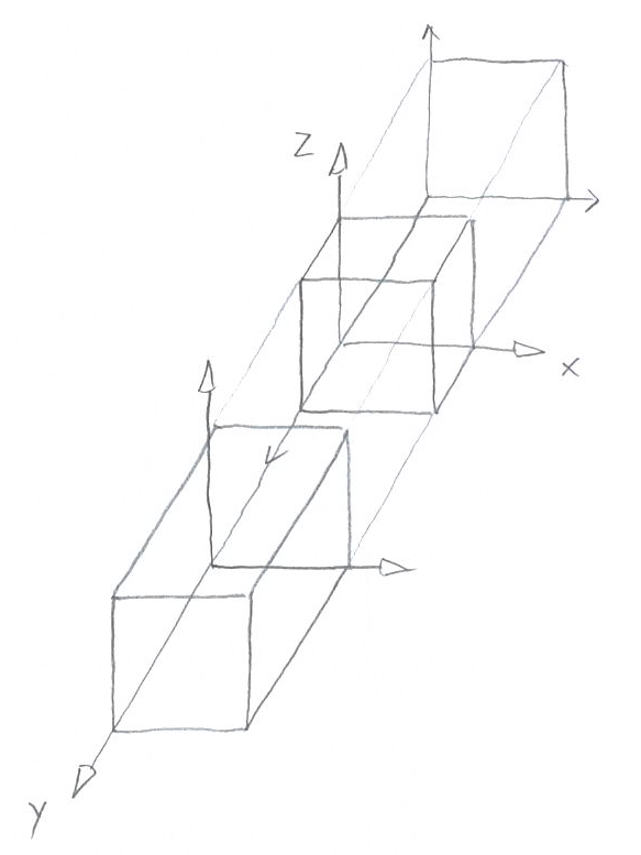
Nevertheless, architecture conventions set a frame of how oblique projections are used and the add-on implements oblique projection according to its applications in architectural drawings. These follow mostly a rather simple principle: the position of the projection plane is parallel to a main face of the 3D object. The result of this position is that the selected face will be projection without any deformations.
This convention results in a setting in which the reduction coefficients of two axes remain at 1 and the third coefficient is variable. For the oblique cases, the Pohlke oblique projection exposes this parameter. The plane can be positioned according to the alpha/beta angles and the reduction coefficient of the projected axis can be modified.